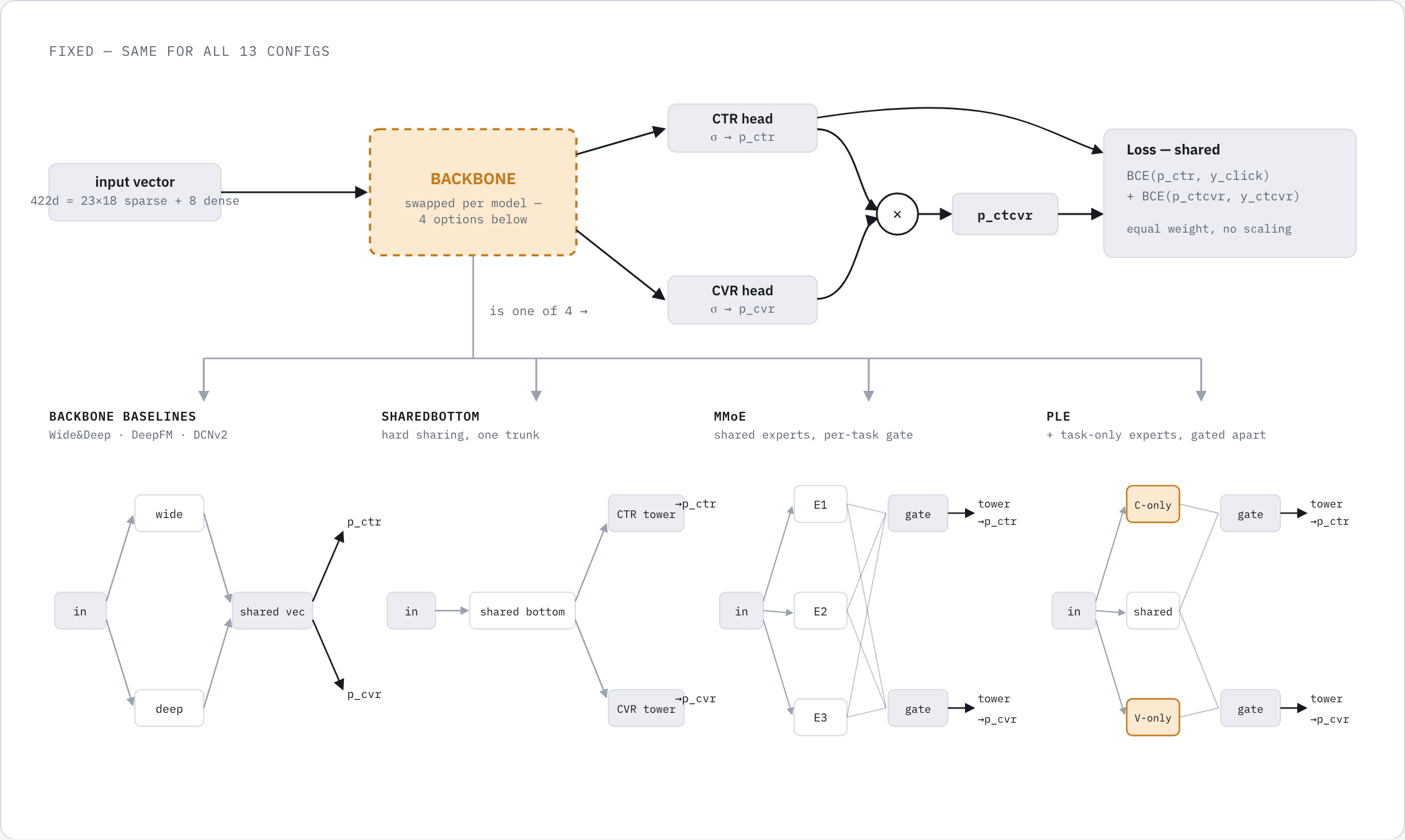
Here we conducted the experiments using the popular multi-task learning models and compare their performance.

Dataset

We used the Ali-CCP dataset for the experiments here. The details of the dataset has been introduced here.

Dataset processing

The Ali-CCP dataset would be first processed by the processing code here so that we have the artifacts having joined features for each impression and ready to be loaded for training.

1. extract.py: Extract the compressed file (.tar.gz) into .csv
2. data.py part 1: parse_raw_ali_ccp_streaming_write
   1. First read the common-features csv file and create a dictionary of mapping the common feature key to the stored common features
   2. Read the skeleton file by chunks size 500K rows
   3. For each read chunk, for each row in the chunk, compose the per impression features by joining the common features and the features stored in the skeleton
   4. Write the results to parsed_{train, test}_rows_full.parquet
3. data.py part 2: load_or_biuld_sparse_vocabs_filtered_parquet, stream_normalize_parquet
   1. For the field feat which is a sparse field of string, we need to build the vocabulary to keep only the high frequency value of that field and treat the rest as <UNK> and map to the vocabulary index 0
      1. For implementation detail, we keep feat that appears at least 5 times
   2. The val associated with the feat will not be touched. For example, if there is a row with: field_id: 109_14, feat: “Electronic”, val: 25: the “Electronic” would be converted to <UNK> if it is not high frequency while the val 25 information would still get into the feature
   3. Normalization: for the dense feature val: 25 part, we would apply log1p(abs(x)) * sign(x) compressing the long tail
   4. The above is using the training dataset only, test dataset never get involved
   5. The output is preprocessed_{train, test}.parquet along with vocab which has 23 entries for each field id in the form like vocab["109_14"] = {"sport": 1, "electronics": 2, ...}
      1. The feat in the preprocessed_{train, test}.parquet is still raw string at the step
4. encode.py
   1. This part is loaded every time the training is started. It is the doing the tensorizing
   2. For sparse columns, it would map the string value to an embedding index through vocabulary
   3. For dense value, map it to float32
   4. In the experiments, we have 23 sparse fields and 8 dense fields
   5. For label, map it to float32

Models

On the modeling side, we want to know what gains could the MTL architectures brings compared to those classic RecSys models. The experiments are designed as keeping the model architecture the only variable, other setups are the same. For the classic RecSys models, we do some tweaking to make it able to be used in the same training setup

The involved models are

1. Wide&Deep
   1. Deep module has two heads, one is deep_ctr and the other is deep_cvr
   2. For the wide module, we have one wide module for ctr and another for cvr (wide_ctr, wide_cvr)
   3. logit_ctr = wide_ctr + deep_ctr; logit_cvr = wide_cvr + deep_cvr
   4. p_ctcvr = sigmoid(logit_ctr) * sigmoid(logit_cvr)
   5. Implementation here
   6. Caveat: Here the wide implementation does not use the cross operation which could have impacts on the performance. Also how to combine the deep scores and the wide scores should be more sophisticated. This is a follow up experiment
2. DeepFM
3. DCNv2
4. Shared bottom
5. MMoE
6. PLE